Metrics for General Circulation Model Evaluation
Tropical El Niño Southern Oscillation Anomaly Database (TEAD)
Overview: This Tropical El Niño Southern Oscillation (ENSO) Anomaly Database contains information on the tropical atmospheric response to El Niño events using various NASA satellite measurements and NCEP/NCAR Reanalysis 1 product. The tropical ENSO signal spreads to remote regions through atmospheric teleconnection mechanisms. The method used to define the ENSO anomaly at any location is based on the assumptions that the ENSO phase can be represented by the Niño 3.4 index and that there exist stable global linear lag/lead relationships between the Niño 3.4 index and climate parameters elsewhere. Chen et al (2008) (see their appendix A) demonstrate that the 6-year high-pass filtered Niño-3.4 index (N34h) and the extreme cross correlation with the least lag (ECLL) between the N34h index and a given climate parameter provides a good approximate description of the ENSO effect on that parameter. Thus the ENSO anomaly can be obtained at the grid box level from the spatiotemperal field of any parameter by regressing the parameter onto the N34h index for the least lag at which the extreme cross-correlation magnitude occurs. This method can be used in two ways: 1) to remove the ENSO signal from a given climate field and isolate longer time scale variability (e.g., Chen et al 2008); 2) to obtain the ENSO signal from a given climate field (e.g. Chen et al 2007) to evaluate general circulation model (GCM) simulations of the atmopsheric response to prescribed time-varying sea surface temperatures.
This project is supported by NASA funding from the American Recovery and Reinvestment Act of 2009.
Chen, J., A.D. Del Genio, B.E. Carlson, and M.G. Bosilovich, 2008: The spatiotemporal structure of twentieth-century climate variations in observations and reanalyses. Part I: Long-term trend. J. Climate, 21, 2611-2633, doi:10.1175/2007JCLI2011.1.
Chen, Y., A.D. Del Genio, and J. Chen, 2007: The tropical atmospheric El Niño signal in satellite precipitation data and a global climate model. J. Climate, 20, 3580-3601, doi:10.1175/JCLI4208.1.
Documentation: We follow the procedure described in the above two references, and extract the monthly mean ENSO anomaly from various climate fields to create this database. A list of satellite instruments and corresponding climate fields used to obtain the monthly mean ENSO anomaly are listed here. All data are provided at 2.5x2.5 degree spatial resolution in binary format. The temporal coverage of the database currently extends from Dec. 1997 to Feb. 2009 except for AMSR-E (Jun. 2002 - Feb. 2009), AIRS (Sep. 2002 - Feb. 2009) and ISCCP (Sep. 1996 - Dec. 2007). For a detailed list of observational data files, click here. To facilitate extraction of the equivalent ENSO anomaly fields from GCM output, software written in Fortran and KornShell is provided with this database distribution. The observational ENSO monthly mean anomaly data and the software to obtain the equivalent anomalies from GCM output are available through our ftp server. (See the README files for more details on data format, sample reading program etc.).


Example: The top-left figure shows an example of the sea surface temperature (SST) ENSO anomaly field obtained by applying this technique to Tropical Rainfall Measuring Mission (TRMM) Microwave Imager (TMI) data. This demonstrates its ability to capture known features of the ENSO evolution of SST ( Klein et al 1999). The peak and decline of the strong type-I 1997/98 El Niño are clearly shown in this figure: a positive SST anomaly expanding from the date line to the east Pacific, and a negative SST anomaly over the west Pacific and the subtropics in both hemispheres; the anomalies begin to decay in boreal spring 1998. A La NiNinantilde;a appears in boreal autumn 1998 with a negative SST anomaly over the central-eastern Pacific and a positive anomaly over the west Pacific, persisting through boreal winter 2001. The top-right figure shows the corresponding precipitation anomaly field from TRMM TMI data. The ENSO-induced precipitation patterns are characterized by a positive anomaly over the central and eastern Pacific, and a negative anomaly over the western Pacific and the Maritime Continent during El Niño, and vice versa during La Niña. Positive Pacific rainfall anomalies are less extensive than SST anomalies. Rainfall decreases during the warm phase in the climatological intertropical convergence zone (ITCZ) and South Pacific convergence zone locations, including the east Pacific ITCZ where SST warms. Positive Indian Ocean (IO) rainfall anomalies occur during the warm phase, but only in the western part of the basin, while SST warms over most of the IO.
Extended ISCCP Tropical Weather State Classification Dataset
Overview: This dataset contains the classified tropical weather states (i.e. cloud regimes) for each grid box (2.5x2.5) within the region of -15N to +15N for the period of Jan. 1, 2005 to Jun. 30, 2007 using ISCCP cloud top pressure - optical depth histogram data. It is the extension of the already available classification (see the figure below, Example 1) for the previous period (1984-2004) based on a k-means clustering analysis (Rossow et al. 2005). For the previous period dataset and details on the methodology, please follow this link. This multi-year database of 3-hourly gridded ISCCP weather state classification can be used to examine the cloud regime shifts in response to various mode of large-scale temporal and/or spatial variability such as the Madden-Julian Oscillation (MJO) (e.g. Chen and Del Genio 2009), ENSO, and the diurnal cycle. It can also be combined with other datasets, e.g. to compare passive remote sensing retrievals of cloud vertical structure to active remote sensing retrievals from the ground (ARM/ASR) or from satellite (CloudSat-Calipso).
This project is supported by NASA funding from the American Recovery and Reinvestment Act of 2009.
![]()
Chen, Y. and A.D. Del Genio, 2009: Evaluation of tropical cloud regimes in observations and a general circulation model. Clim. Dynam., 32, 355-369, doi:10.1007/s00382-008-0386-6.
Documentation: For detailed information about the data files, please see README. The extended data and software to read and convert to equal angle coordinates are available through our ftp server.
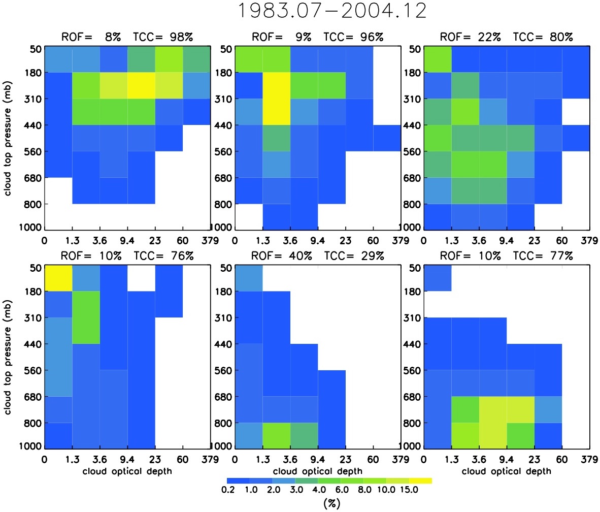
Example 1: The figure above shows the 6 weather states identified by k-means clustering of the ISCCP cloud top temperature-optical thickness diagrams. The top panel represents the more disturbed cloud regimes, loosely corresponding to (left) deep convection, (middle) cirrostratus anvil, and (right) middle-level cumulus congestus states. The bottom panel represents the more suppressed cloud regimes, loosely corresponding to (left) isolated cirrus, (middle) shallow trade cumulus, and (right) marine stratocumulus.


Example 2: The left figure above shows an example of using ISCCP weather state classification to depict MJO propagation over the tropical ocean. The six ISCCP weather states, color-coded from red to violet, correspond to deep convection, cirrostratus anvils, mid-level cumulus congestus, isolated cirrus, shallow trade cumulus and marine stratocumulus. In this Hovmoller diagram, eastward propagation of the deep convection states (red) with a period of ~30 days is clearly visible, suggestive of the MJO. The right figure above shows composite relative frequency of occurrence (RFO) bar-charts for each state as a function of MJO phase. It was constructed using the classification indices at seven lag periods in pentads for the region from 60E to 180E within +/-5N. Lag 0 refers to a period of +/-2.5 days around the MJO peak phase. Negative lag is defined as the longitude zones east of the MJO peak, i.e. preceding it in time. The coherent progression of the ISCCP weather states during passage of MJO events is clearly shown: the RFOs of the deep convective (red) and the anvil (orange) states increase significantly approaching the peak phase of MJOs and reach their maxima at the peak phase; then the deep convection decreases immediately while the anvil state remains for another 5 days or so and decreases gradually afterwards; the mid-level congestus (yellow) and shallow cumulus (blue) states dominate several weeks before the MJO peak, decreasing (increasing) before (after) the peak; the RFO of the cirrus state (green) is almost constant with MJO phase, suggesting that the presence of isolated cirrus in this tropical region is ubiquitous and not associated with convective activity (Chen and Del Genio 2009).

Example 3: The figure above shows the CloudSat-CALIPSO all-level cloud composites for the 6 ISCCP weather states (C1 - C6) based on Jan. 2007 data. The deep convection state (C1) contains a significant amount of clouds through the whole column of the troposphere, while all other states have a bimodal distribution. The altitudes of the peak in the upper troposphere are lower in the convectively active states (C1-C3) compared to those in the convectively suppressed states (C4-C6). The 3 convective states also have much more mid-level cloud than the 3 suppressed states do.

Example 4: The composite diurnal cycle of the 6 weather states over three tropical regions are shown above as an example (Top: Tropical Western Pacific (TWP); Middle: Amazon region; Bottom: Equatorial Africa (EAF)) based on one year ISCCP classification data from Jul. 2006 to Jun. 2007. Only the daytime fraction of the diurnal cycle is shown because the regime definitions require visible optical thickness information. The Y-axis represnts the relative frequency of occurrency (RFO) of each state during a time period, which is labeled as center local time during this time period along the X-axis. The deep convection state (C1) peaks in early afternoon in the TWP region and in late afternoon over the other two tropical land regions. In all 3 regions, the anvil state (C2) has two peaks: one in early morning and another in late afternoon. The middle level congestus (C3) peaks in either late morning or ealy afternoon depending on the region. In TWP region, the isolated cirrus state (C4) has early morning and late afternoon peaks, while in Equatorial Africa a single midday peak is observed and in the Amazon isolated cirrus are rare. The shallow cumulus state (C5) is most common in midday in the TWP and Amazon regions but has little diurnal cycle in Equatorial Africa. The stratocumulus state (C6) is rare in all three regions, as are totally clear skies.
Weather Research and Forecasting (WRF) cloud-resolving model simulation diagnostics
Overview: This dataset contains the model output from a WRF V2.2 cloud-resolving simulation (with 1.33 km horizontal resolution) of tropical convection near Darwin, Australia during the intensive observing period of the Tropical Warm Pool - International Cloud Experiment (TWP-ICE). Provided here are 10-minute resolution model outputs from simulations of the two distinctive convective regimes during TWP-ICE: an active monsoon period with storms somewhat like those typical of a maritime environment (0Z 1/20/2006 - 12Z 1/22/2006); and a monsoon break period with occasional strong continental-type convection (0Z 2/10/2006 - 12Z 2/12/2006). This dataset can be used to study the differences between different convective regimes (e.g., Wu et al. 2009). Combined with observations, it can also be used to evaluate the convection parameterization in General Circulation Models (GCMs) or as a tool for the development of new parameterization.
This project is supported by NASA funding from the American Recovery and Reinvestment Act of 2009.
![]()
Wu, J., A.D. Del Genio, M.-S. Yao, and A.B. Wolf, 2009: WRF and GISS SCM simulations of convective updraft properties during TWP-ICE. J. Geophys. Res., 114, D04206, doi:10.1029/2008JD010851.
Documentation: For detailed information about the dataset, please see README. The dataset is in netcdf format. Click here for the header information. The full dataset is available to download from our ftp server. Since the size of the entire dataset is very large, plots of time series of the domain mean precipitation and cloud fraction are provided as a reference for users who may wish to download some fraction of the dataset in which they might be interested (see figures below).

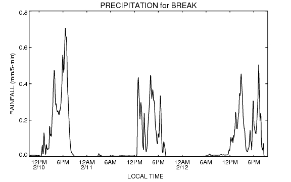
Precipitation Figures: The precipitation plots (left panel for active period; right panel for break period) give the rainfall rate over a 5-min accumulation (in units of mm/5-min, where 5-min is the model output frequency). They show 3 clear diurnal cycles during the 2.5 day simulation, with precipitation mainly produced between 12pm-9pm local time.
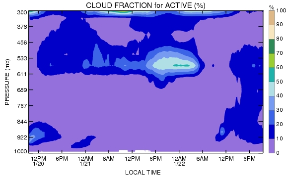

Cloud Fraction Figures: The cloud fraction is calculated as the percentage ratio of the number of cloudy grid boxes to the number of total grid boxes in the domain. Cloudy grids are defined as (QCLOUD+QICE)>1.e-6 kg/kg, where QCLOUD is the mixing ratio of cloud water and QICE is the mixing ratio of cloud ice. For the active monsoon period (left panel), convection is widespread and clouds exist almost everywhere anytime. For the monsoon break period (right panel), the convection mainly exists in the afternoon when the land surface has been heated by incident sunlight.
